  b.var = function(d, i){
                           var(d[i])
}Homework 9: Bootstrapping (Solutions)
Create a b.var function
I’m lazy and will use the boot package to run my bootstrap. I need a function that computes the variance that can be passed to the boot function.
Create a dataset of 100 normal observations
args(rnorm)function (n, mean = 0, sd = 1)
NULL n = 100
mu = 2
sig = 7
normal_data = rnorm(n, mu, sig)
write.csv(normal_data, "hw9_normal_data.csv")
c(summary(normal_data), var_x=var(normal_data), sd_x=sd(normal_data)) Min. 1st Qu. Median Mean 3rd Qu. Max. var_x
-17.657899 -2.815995 2.841938 2.318169 8.607117 20.758200 68.992901
sd_x
8.306197 Bootstrap the variance using b.var
  ### Use the boot function to run the bootstrap
  normal_b.var = boot(normal_data, b.var, R=9999)
  normal_b.var
ORDINARY NONPARAMETRIC BOOTSTRAP


Call:
boot(data = normal_data, statistic = b.var, R = 9999)


Bootstrap Statistics :
    original     bias    std. error
t1*  68.9929 -0.6638074    9.491217
How much bias does the estimate have? Is the bootstrap distribution normal or chisquare?
attributes(summary(normal_b.var))$names
[1] "R" "original" "bootBias" "bootSE" "bootMed"
$row.names
[1] 1
$class
[1] "summary.boot" "data.frame" summary(normal_b.var) R original bootBias bootSE bootMed
1 9999 68.993 -0.66381 9.4912 67.934 plot(normal_b.var)
qqPlot(normal_b.var$t, distribution="norm")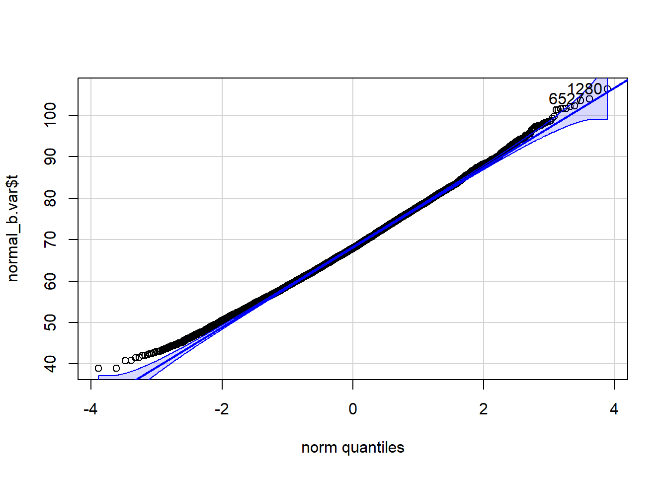
[1] 1280 6527 qqPlot(normal_b.var$t, distribution="chisq", df=n-1)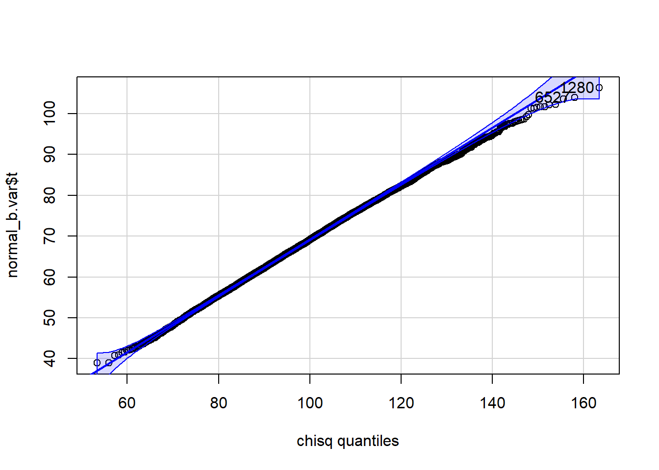
[1] 1280 6527The variance estimator appears to have bias=-0.6638074 and SE=9.491217 when the data consist of 100 observations randomly drawn from a normal with mean \mu= 2 and variance \sigma^2= 49. The variance appears to be neither normally nor chisquare distributed, although the chisquare may fit a bit better.
Create a dataset of 100 standard normal observations
args(rnorm)function (n, mean = 0, sd = 1)
NULL n = 100
mu = 0
sig = 1
std_normal_data = rnorm(n, mu, sig)
write.csv(std_normal_data, "hw9_std_normal_data.csv")
c(summary(std_normal_data), var_x=var(std_normal_data), sd_x=sd(std_normal_data)) Min. 1st Qu. Median Mean 3rd Qu. Max.
-3.01615267 -0.68727954 0.02286484 -0.01098460 0.79788373 2.28271992
var_x sd_x
1.20641306 1.09836836 Bootstrap the variance using b.var
  ### Use the boot function to run the bootstrap
  std_normal_b.var = boot(std_normal_data, b.var, R=9999)
  std_normal_b.var
ORDINARY NONPARAMETRIC BOOTSTRAP


Call:
boot(data = std_normal_data, statistic = b.var, R = 9999)


Bootstrap Statistics :
    original      bias    std. error
t1* 1.206413 -0.01230282   0.1569296
How much bias does the estimate have? Is the bootstrap distribution normal or chisquare?
summary(std_normal_b.var) R original bootBias bootSE bootMed
1 9999 1.2064 -0.012303 0.15693 1.1899 plot(std_normal_b.var)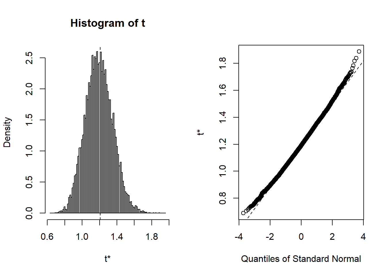
qqPlot(std_normal_b.var$t, distribution="norm")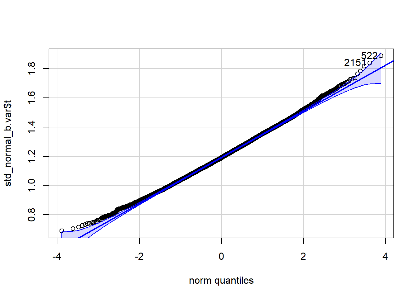
[1] 522 2151 qqPlot(std_normal_b.var$t, distribution="chisq", df=n)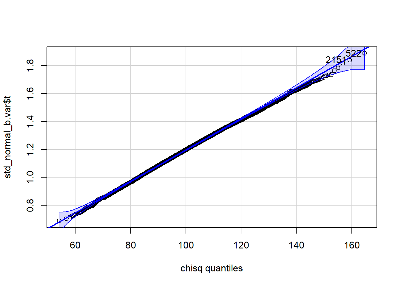
[1] 522 2151The variance estimator appears to have bias=-0.0123028 and SE=0.1569296 when the data consist of 100 observations randomly drawn from a normal with mean \mu= 0 and variance \sigma^2= 1. The variance appears not to be normally distributed. However, it appears to have a chisquare distribution. The MGF of the sum of squared standard normals supports this contention.
Create a dataset of 100 U(0,1)
args(rnorm)function (n, mean = 0, sd = 1)
NULL n = 100
a = 0
b = 1
unif_data = runif(n, a, b)
write.csv(unif_data, "hw9_unif_data.csv")
c(summary(unif_data), var_x=var(unif_data), sd_x=sd(unif_data)) Min. 1st Qu. Median Mean 3rd Qu. Max.
0.0008975214 0.2545879553 0.5409294020 0.5118967322 0.7402595778 0.9963748557
var_x sd_x
0.0798313631 0.2825444445 Bootstrap the variance using b.var
  ### Use the boot function to run the bootstrap
  unif_b.var = boot(unif_data, b.var, R=9999)
  unif_b.var
ORDINARY NONPARAMETRIC BOOTSTRAP


Call:
boot(data = unif_data, statistic = b.var, R = 9999)


Bootstrap Statistics :
      original       bias    std. error
t1* 0.07983136 -0.000820566 0.007331027
How much bias does the estimate have? Is the bootstrap distribution normal or chisquare?
summary(unif_b.var) R original bootBias bootSE bootMed
1 9999 0.079831 -0.00082057 0.007331 0.078908 plot(unif_b.var)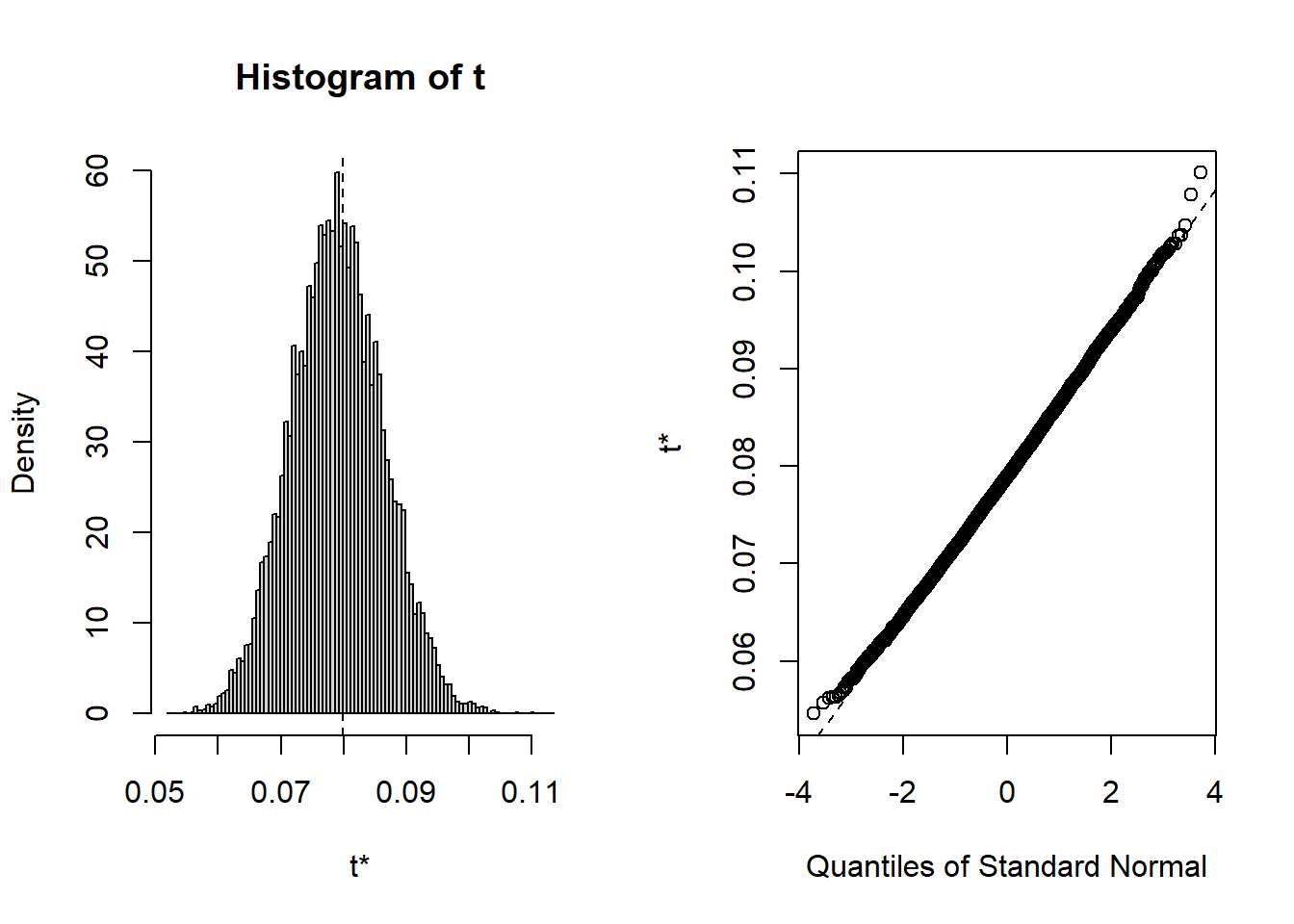
qqPlot(unif_b.var$t, distribution="norm",)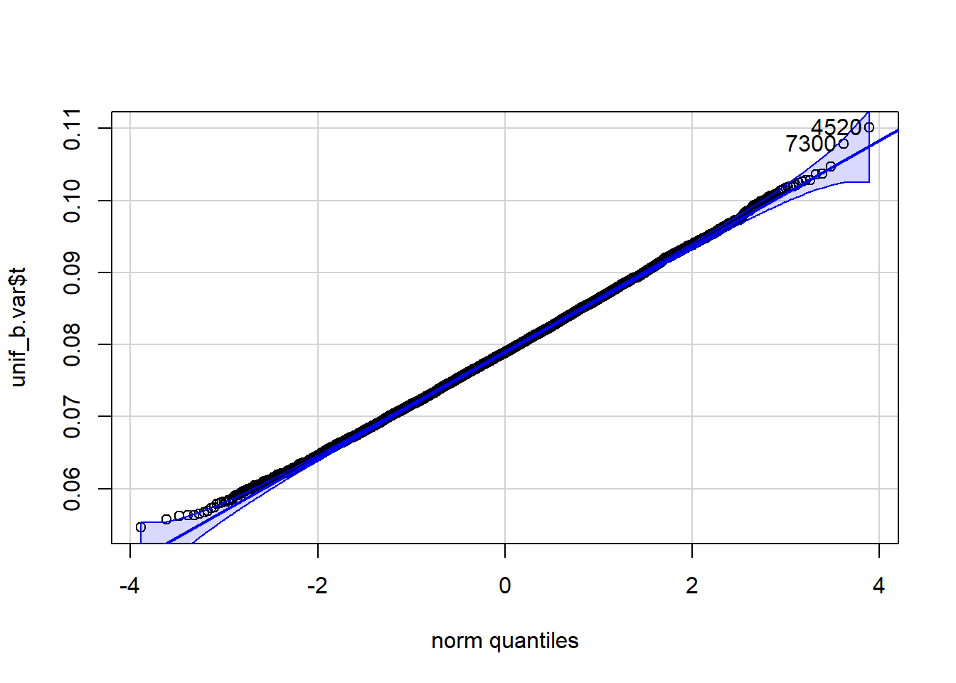
[1] 4520 7300 qqPlot(unif_b.var$t, distribution="unif", min=a, max=b)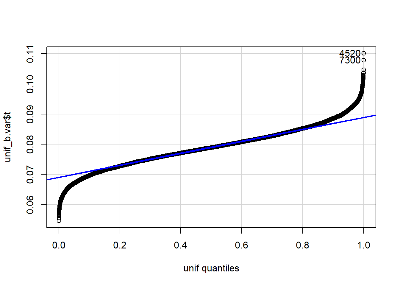
[1] 4520 7300 qqPlot(unif_b.var$t, distribution="beta", shape1=(3*n-1)/2, shape2=(3*n-1)/2)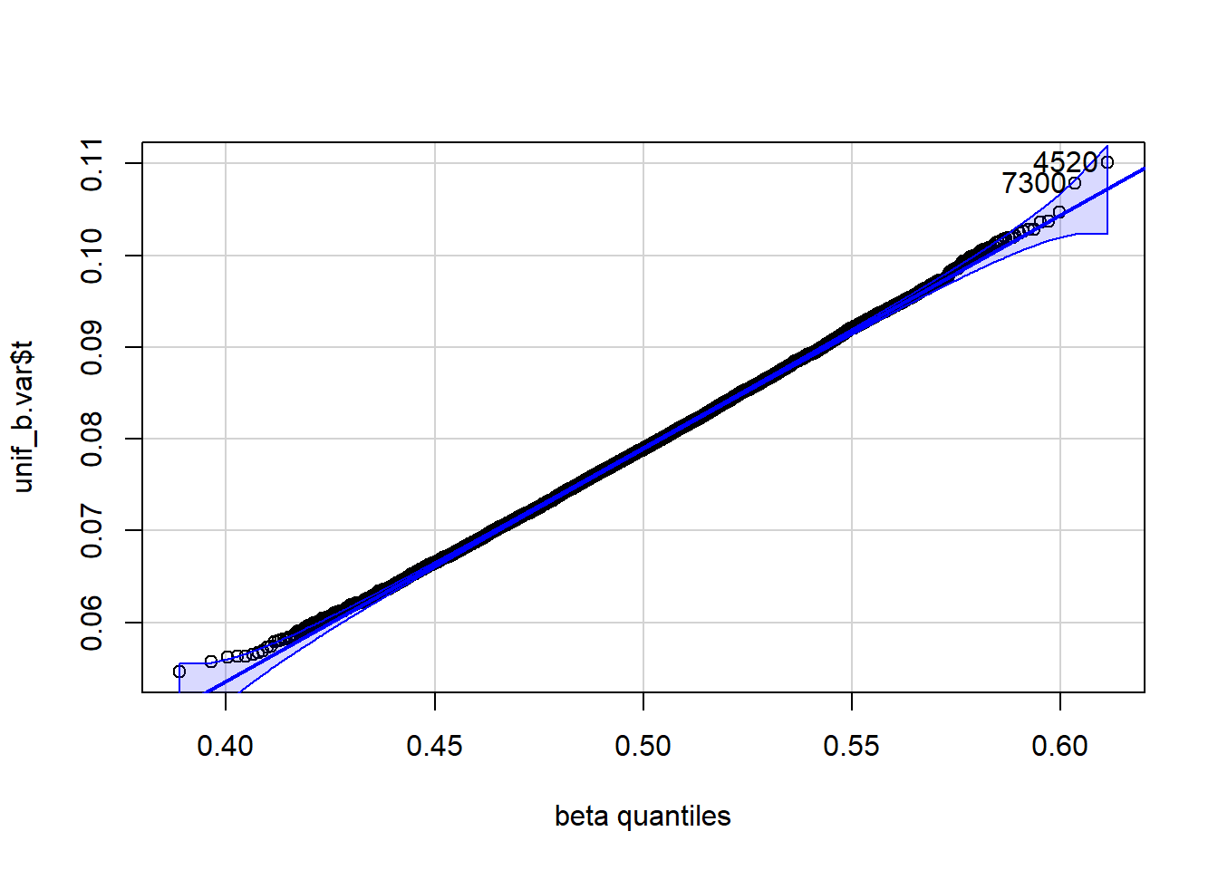
[1] 4520 7300When the data consist of 100 observations randomly drawn from a U( 0 , 1), the variance estimator appears to be unbiased as bias=-8.20566^{-4}. The standard error is SE=0.007331. The variance appears to be somewhat normally distributed, but it is not U( 0 , 1) distributed. For appropriately chosen shape parameters, \alpha and \beta, the distribution of the variance appears to be almost beta.